Air-to-air Heat Exchanger Heat Transfer Calculation Methodology and CalculatorCalculation

Introduction

This calculation methodology is based on the 2020 ASHRAE Handbook – Systems and Equipment, Chapter 26. The calculator is used to estimate a full year of sensible and latent heat transfer in an energy recovery ventilation (ERV) system. This methodology assumes that the air handling unit (AHU) uses a variable speed supply fan, and that the energy recovery component is a rotary wheel. Figure 1 shows an example of an ERV system.

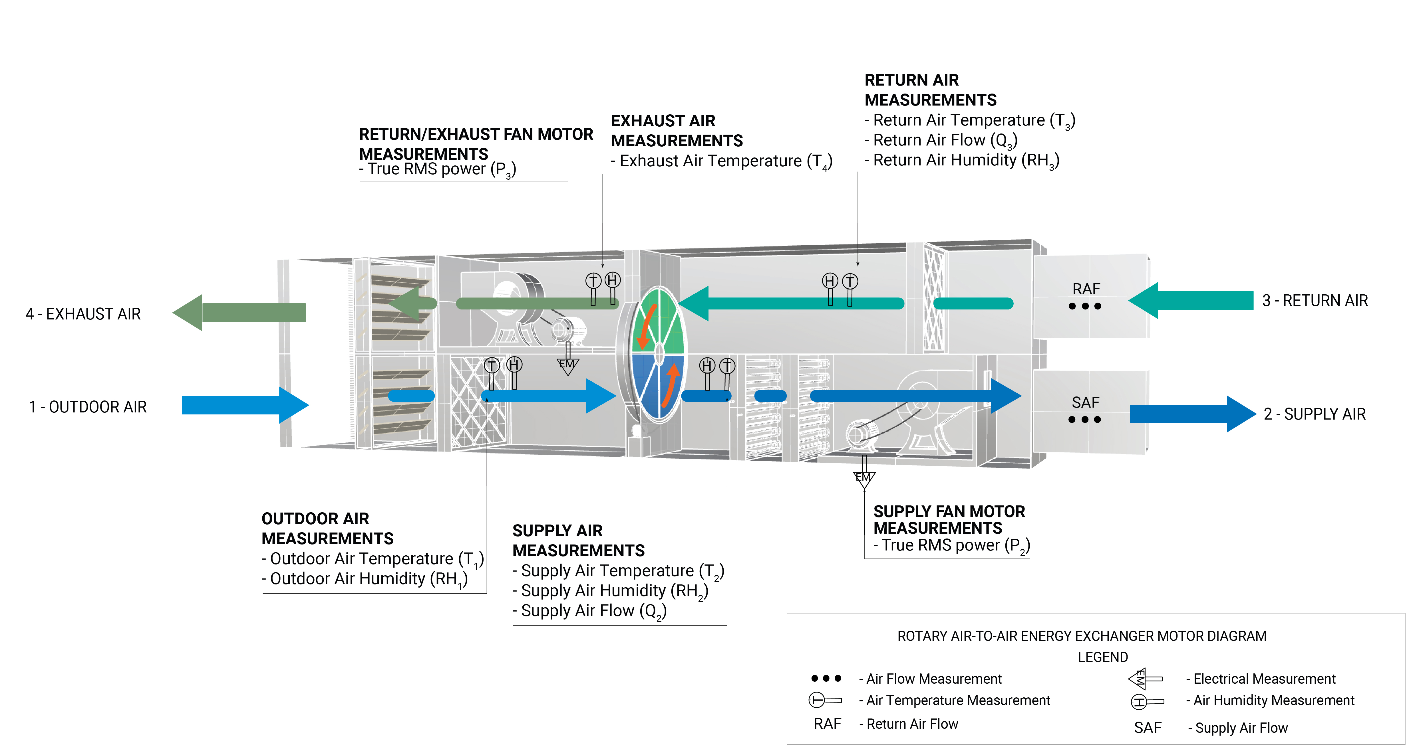
This methodology works with hourly data only and each measurement is taken at the start of the hour for a minimum duration of six weeks. If the ERV system is used during both the heating and cooling seasons, then six weeks of data per season is needed. Data is used to calculate heat transfer for the measurement period first, then is extrapolated to a full year. Measurement points are shown in Figure 2 and the variables to measure are listed in Table 2.

Section A.1 describes how to calculate the sensible and latent heat transfer for the duration of the measurement period. If six weeks of data is collected, then heat transfer will be calculated for each hour interval for those six weeks. Sensible and latent effectiveness are a measure of the performance of the ERV system. Effectiveness is the actual heat transfer divided by the maximum possible heat transfer by the heat exchanger. These values are calculated in section A.1 for each hour interval and are used in section A.2 to estimate the full-year heat transfer.

To calculate latent heat transfer and effectiveness, first the humidity ratio $(lb_m/lb_m)$ must be calculated. Table 1 summarizes the equations used to determine humidity ratio for a given relative humidity value. The calculator selects the appropriate equation based on the measured hourly relative humidity and then uses the measured hourly temperature to run the calculation (CUNY BPL BRT, 2022, pp. 22). The equations in Table 1 result in a humidity ratio with units of grains of water per pound of dry air (grains/lb). The calculator performs an additional calculation to convert the units of grain/lb to $lb_m/lb_m$.

Where,

$T =$ hourly measured air temperature of the respective air stream (F)

$W_g =$ humidity ratio (grains/lb)

To estimate heat transfer for a full year, simple linear regression (used to assess the relationship between two variables) is performed in Microsoft Excel using the LINEST function. These calculation steps are described in more detail in Section A.2.

Section A.3 describes how to calculate the electrical energy consumption of the supply and return fan motors using hourly power draw data. The hourly data is used to develop an average hourly schedule of both fan motors for all seven days of the week as a proxy of the occupancy schedule of the facility. This occupancy schedule is used in Section A.2 to conduct the simple linear regressions.

Calculator

Air-to-air Heat Exchanger Calculations

A.1: Heat Transfer for the Measurement Period

The following methodology is used to calculate the sensible and latent heat transferred by the ERV system during the measurement period only. Sensible and latent effectiveness are also calculated in this process. All data used in section A.1 should rely on data being measured with either data loggers or BMS historical trends. Measured data used in this section is summarized in Table 3.

1. Calculate the mass flow rate of supply air leaving the ERV for each hour interval.

\begin{equation} \dot{m_2} = Q_2/v \end{equation}

Where,

$\dot{m_2} =$ hourly mass flow rate of supply air leaving the ERV (lb$_m$/min)

$Q_2 =$ hourly air flow rate of supply air leaving the ERV (ft$^3$/min)

$v =$ specific volume of air, 12.49 (ft$^3$/lb)

2. Calculate the mass flow rate of return air entering the ERV for each hour interval.

\begin{equation} \dot{m_3} = Q_3/v \end{equation}

Where,

$\dot{m_3} =$ hourly mass flow rate of return air entering the ERV (lb$_m$/min)

$Q_3 =$ hourly air flow rate of return air entering the ERV (ft$^3$/min)

$v =$ specific volume of air, 12.49 (ft$^3$/lb)

3. Calculate the humidity ratio for outside air entering the ERV ($W_1$), supply air leaving the ERV ($W_2$) and return air entering the ERV ($W_3$) for each hour interval. In this step, the measured hourly temperature and relative humidity data of the respective air stream is used with the equations in Table 1 to determine the humidity ratio for that hour. In this same step, the units are converted from grains/lb to lb$_m$/lb$_m$.

\begin{equation} W_n = 0.000142857 * W_g \end{equation}

Where,

$W_n =$ humidity ratio of a given air stream (lb$_m$/lb$_m$)

$0.000142857 =$ constant value, (lb$_m$/lb$_m$)

$W_g =$ humidity ratio calculated from Table 1

4. Calculate sensible heat transferred by the ERV for each hour interval.

\begin{equation} q_s = \dot{m}_2c(T_1 - T_2) \end{equation}

Where,

$q_s =$ sensible heat transferred by the ERV each hour (Btu/h)

$c =$ specific heat of air at normal atmospheric pressure, 0.243 (Btu/lb F)

$\dot{m}_2 =$ hourly mass flow rate of supply air leaving the ERV (lb$_m$/min)

$T_1 =$ hourly temperature of outside air entering the ERV (F)

$T_2 =$ hourly temperature of supply aire leaving the ERV (F)

5. Calculate latent heat transferred by the ERV for each hour interval.

\begin{equation} q_L = \dot{m}_2h(W_1 - W_2) \end{equation}

Where,

$q_L =$ latent heat transferred by the ERV each hour (Btu/h)

$h =$ latent heat of vaporization, 970.1 (Btu/lb)

$\dot{m}_2 =$ hourly mass flow rate of supply air leaving the ERV (lb$_m$/min)

$W_1 =$ hourly humidity ratio of outside air entering the ERV (lb$_m$/lb$_m$)

$W_2 =$ hourly humidity ratio of supply air leaving the ERV (lb$_m$/lb$_m$)

6. Heat transfer should be calculated only when the energy/heat recovery mode is on. This can be determined by checking the temperature difference across the recovery system in both the supply-air side and the return-air side. Another condition is that the supply fan motor must be running for heat transfer to occur. Sometimes the ERV is off and the supply fan motor is on, in this scenario we cannot assume heat transfer occurs.

\begin{equation} \text{If} \hspace{2mm} \begin{cases} T_1 - T_2 > 1 & \text{heat transfer during cooling season}\\ T_1 - T_2 < -1 & \text{heat transfer during heating season} \\ -1 < T_1 - T_2 < 1 & \text{no heat transfer occurs} \end{cases} \end{equation}

Where,

$T_1 =$ measured hourly temperature of outside air entering the ERV (F)

$T_2 =$ measured hourly temperature of supply air leaving the ERV (F)

\begin{equation} \text{If} \hspace{2mm} \begin{cases} T_3 - T_4 > 1 & \text{heat transfer during cooling season}\\ T_3 - T_4 < -1 & \text{heat transfer during heating season} \\ -1 < T_3 - T_4 < 1 & \text{no heat transfer occurs} \end{cases} \end{equation}

Where,

$T_3 =$ measured hourly temperature of return air entering the ERV (F)

$T_4 =$ measured hourly temperature of exhaust air leaving the ERV (F)

\begin{equation} \text{If} \hspace{2mm} \begin{cases} Q_2 > 0 & \text{heat transfer occurs}\\ Q_2 < 0 & \text{no heat transfer occurs} \end{cases} \end{equation}

Where,

$Q_2 =$ air flow rate of supply air leaving the ERV (ft$^3$/min)

\begin{equation} \text{If} \hspace{2mm} \begin{cases} Q_3 > 0 & \text{heat transfer occurs}\\ Q_3 < 0 & \text{no heat transfer occurs} \end{cases} \end{equation}

Where,

$Q_3 =$ air flow rate of return air entering the ERV (ft$^3$/min)

Sensible and Latent Heat Effectiveness

Sensible and latent heat effectiveness has the same conditions as heat transfer where effectiveness should be calculated only when the energy/heat recovery mode is on and the supply fan motor must be running.

1. Calculate the latent effectiveness for each hour interval.

\begin{equation} \varepsilon_L = \frac{\dot{m}_2h(W_1 - W_2)}{\dot{m}_{min}h(W_1 - W_3)} \end{equation}

Where,

$\varepsilon_L =$ hourly latent effectiveness of the ERV

$h =$ latent heat of vaporization, 970.1 (Btu/lb)

$\dot{m}_2 =$ hourly mass flow rate of supply air leaving the ERV (lb$_m$/min)

$\dot{m}_{min} =$ minimum hourly mass flow rate value (lb$_m$/min)

$W_1 =$ hourly humidity ratio of outisde air entering the ERV (lb$_m$/lb$_m$)

$W_2 =$ hourly humidity ratio of supply air leaving the ERV (lb$_m$/lb$_m$)

$W_3 =$ hourly humidity ratio of return air entering the ERV (lb$_m$/lb$_m$)

2. Calculate the sensible effectiveness for each hour interval.

\begin{equation} \varepsilon_s = \frac{\dot{m}_2c(T_1 - T_2)}{\dot{m}_{min}c(T_1 - T_3)} \end{equation}

Where,

$\varepsilon_s =$ hourly sensible effectiveness of the ERV

$c =$ specific heat of air at normal atmospheric pressure, 0.243 (Btu/lb F)

$\dot{m}_2 =$ hourly mass flow rate of supply air leaving the ERV (lb$_m$/min)

$\dot{m}_{min} =$ minimum hourly mass flow rate value (lb$_m$/min)

$T_1 =$ hourly temperature of outisde air entering the ERV (F)

$T_2 =$ hourly temperature of supply air leaving the ERV (F)

$T_3 =$ hourly temperature of return air entering the ERV (F)

A.2: Heat Transfer for the Full Year

To estimate the full year heat transfer, the occupancy patterns and schedule defined in the measurement period are extrapolated to the entire year. Supply air flow (Q2), return air flow (Q3), and sensible and latent effectiveness are calculated by performing a regression analysis with the variables listed in Table 4. Regression analysis plots data on a graph and generates a line that traces the distribution of data. The line has a formula associated with it and the formula is used to project the dependent variable for the full year. To accomplish this, the Microsoft Excel function LINEST is used with the values in Table 4.

Regressions 1 and 2

There is a cubic relationship between fan motor draw and air flow rate. The equation that describes the relationship between these variables is:

\begin{equation} y = ax^3 + bx^2 + cx + d \end{equation}

Where,

$y =$ dependent variable at each hour for a full year, the value being projects ($Q_2$ and $Q_3$)

$x =$ independent variable at each hour for a full year, the suply fan motor energy consumption

$a,b,c,d =$ cubic relationship coefficients

With this formula, the air flow rate Q2 and Q3 can be projected for the full year by plugging in values for x, the supply fan motor power draw. This data is the measured power draw of the supply and return fan motors.

Regressions 3 and 4

These steps yield an assessment of the relationship between the measured air flow rate of supply air leaving the ERV system (Q2) and the sensible and latent heat effectiveness that was calculated in section A.1. The relationship between air flow rate and effectiveness is linear and the equation that describes the relationship is:

\begin{equation} y = mx + b \end{equation}

Where,

$y =$ dependent variable at each hour for a full year, the value being projects (sensible and latent effectiveness)

$m =$ slope of the line, generated by Excel

$x =$ independent variable at each hour for a full year, the air flow rate of air leaving the ERV system ($Q_2$)

$b =$ y-intercept of the line generated by Excel

The values of $Q_2$ that were calculated in the previous section are then plugged into Equation (11) to project sensible and latent heat transfer effectiveness for the full year:

\begin{equation} \varepsilon_s = m(Q_2) + b \end{equation}

\begin{equation} \varepsilon_L = m(Q_2) + b \end{equation}

Where,

$\varepsilon_s =$ projected sensible effectiveness

$\varepsilon_L =$ projected latent effectiveness

$Q_2 =$ projected air flow rate of supply air leaving the ERV (ft$^3$/min)

After projecting the airflows and effectiveness rates to a full year, the next step is to calculate the hourly mass flow rates and humidity ratios for a full year.

1. Calculate the mass flow rate of supply aire leaving the ERV for each hour interval for the entire year.

\begin{equation} \dot{m}_2 = Q_2/v \end{equation}

Where,

$\dot{m}_2 =$ hourly mass flow rate of supply air leaving the ERV (lb$_m$/min)

$Q_2 =$ projected hourly air flow rate of supply are leaving the ERV (ft$^3$/min)

$v =$ specific volume of air, 12.49 (ft$^3$/lb)

2. After projecting the airflows and effectiveness rates to a full year, the next step is to calculate the hourly mass flow rates and humidity ratios for a full year.

\begin{equation} \dot{m}_3 = Q_3/v \end{equation}

Where,

$\dot{m}_3 =$ hourly mass flow rate of return air entering the ERV (lb$_m$/min)

$Q_3 =$ projected hourly air flow rate of return air entering the ERV (ft$^3$/min)

$v =$ specific volume of air, 12.49 (ft$^3$/lb)

3. Calculate the humidity ratio for outside air entering the ERV (W1). In this step, the hourly climate normal year (CNY) outside air temperature (OAT) and relative humidity data is used with the equations in Table 1 to determine the humidity ratio for that hour. In this same step, the units are converted from grains/lb to lb$_m$/lb$_m$.

\begin{equation} W_n = 0.000142857 * W_g \end{equation}

Where,

$W_n =$ humidity ratio of a given air stream (lb$_m$/lb$_m$)

$0.000142857 =$ constant value, (lb$_m$/lb$_m$)

$W_g =$ humidity ratio calculated from Table 1

4. Estimate the hourly humidity ratio of supply air leaving the ERV for the full year. In this equation, it is assumed that the latent heat of vaporization is constant.

\begin{equation} W_2 = \frac{\dot{m}_2W_1 - \varepsilon_L\dot{m}_{min}(W_1-W_3)}{\dot{m}_2} \end{equation}

Where,

$W_2 =$ hourly humidity ratio of supply air leaving the ERV (lb$_m$/lb$_m$)

$W_1 =$ hourly humidity ratio of outside air entering the ERV (lb$_m$/lb$_m$)

$W_3 =$ hourly humidity ratio of return air entering the ERV (lb$_m$/lb$_m$)

$\varepsilon_L =$ projected hourly latent effectiveness of the ERV

$\dot{m}_{min} =$ minimum mass flow rate value (lb$_m$/min)

$\dot{m}_2 =$ hourly mass flow rate data of supply air leaving the ERV (lb$_m$/min)

5. Estimate the temperature of supply air leaving the ERV for the full year. In this equation, it is assumed that specific heat of air is constant.

\begin{equation} T_2 = \frac{\dot{m}_2T_1 - \varepsilon_s\dot{m}_{min}(T_1-T_3)}{\dot{m}_2} \end{equation}

Where,

$T_2 =$ hourly temperature of supply air leaving the ERV (F)

$T_1 =$ hourly temperature of outside air entering the ERV (F)

$T_3 =$ hourly temperature of return air entering the ERV (F)

$\varepsilon_s =$ projected hourly sensible effectiveness of the ERV

$\dot{m}_{min} =$ minimum mass flow rate value (lb$_m$/min)

$\dot{m}_2 =$ hourly mass flow rate data of supply air leaving the ERV (lb$_m$/min)

CUNYBPL assumes that T3 and W3 are constant values with the reasoning being that occupants will want the same indoor air temperature regardless of the season. It is up to the heating and cooling plants to maintain that setpoint temperature. The next step is to calculate sensible and latent heat transfer.

6. Calculate sensible heat transferred by the ERV for each hour interval for the full year.

\begin{equation} q_s = \dot{m}_2c(T_1 - T_2) \end{equation}

Where,

$q_2 =$ sensible heat transferred by the ERV each hour (Btu/h)

$c =$ specific heat of air at normal atmospheric pressure, 0.243 (Btu/lb F)

$\dot{m}_2 =$ hourly mass flow rate of supply air leaving the ERV (lb$_m$/min)

$T_1 =$ hourly temperature of outside air entering the ERV (F)

$T_2 =$ hourly temperature of suply air leaving the ERV (F)

7. Calculate latent heat transferred by the ERV for each hour interval for the full year.

\begin{equation} q_L = \dot{m}_2h(W_1 - W_2) \end{equation}

Where,

$q_2 =$ latent heat transferred by the ERV each hour (Btu/h)

$h =$ latent heat of vaporization, 970.1 (Btu/lb)

$\dot{m}_2 =$ hourly mass flow rate of supply air leaving the ERV (lb$_m$/min)

$W_1 =$ hourly humidity ratio of outside air entering the ERV (lb$_m$/lb$_m$)

$W_2 =$ hourly humidity ratio of suply air leaving the ERV (lb$_m$/lb$_m$)

8. Heat transfer should be calculated only when the energy/heat recovery mode is on. This can be determined by checking the temperature difference across the recovery system in both the supply-air side and the return-air side, and air-flow rate across the heat exchanger. Air flow is happening when the supply fan motor and exhaust fan motor are on. Sometimes the ERV rotary wheel is off and air flow bypasses the rotary wheel when the supply fan motor is on, in this scenario we cannot assume heat transfer occurs.

\begin{equation} \text{If} \hspace{2mm} \begin{cases} T_1 - T_2 > 1 & \text{heat transfer during cooling season}\\ T_1 - T_2 < -1 & \text{heat transfer during heating season} \\ -1 < T_1 - T_2 < 1 & \text{no heat transfer occurs} \end{cases} \end{equation}

Where,

$T_1 =$ measured hourly temperature of outside air entering the ERV (F)

$T_2 =$ measured hourly temperature of supply air leaving the ERV (F)

\begin{equation} \text{If} \hspace{2mm} \begin{cases} T_3 - T_4 > 1 & \text{heat transfer during cooling season}\\ T_3 - T_4 < -1 & \text{heat transfer during heating season} \\ -1 < T_3 - T_4 < 1 & \text{no heat transfer occurs} \end{cases} \end{equation}

Where,

$T_3 =$ measured hourly temperature of return air entering the ERV (F)

$T_4 =$ measured hourly temperature of exhaust air leaving the ERV (F)

\begin{equation} \text{If} \hspace{2mm} \begin{cases} Q_2 > 0 & \text{heat transfer occurs}\\ Q_2 < 0 & \text{no heat transfer occurs} \end{cases} \end{equation}

Where,

$Q_2 =$ air flow rate of supply air leaving the ERV (ft$^3$/min)

\begin{equation} \text{If} \hspace{2mm} \begin{cases} Q_3 > 0 & \text{heat transfer occurs}\\ Q_3 < 0 & \text{no heat transfer occurs} \end{cases} \end{equation}

Where,

$Q_3 =$ air flow rate of return air entering the ERV (ft$^3$/min)

A.3: Annual Supply Fan Energy Consumption

This calculation methodology assumes that the power draw of the supply and exhaust fan motors were measured with a power logger at one-hour intervals for a minimum of six weeks. The power logger should have measured the three phases of the panelboard. The following formulas will calculate three phase power first. Next, the calculator reduces the dataset to an hourly schedule for all seven days of the week. This schedule is used to determine when heat transfer occurs. Then, the schedule is extrapolated to a full year and the resultant value is the estimated annual energy consumption of the fan motors.

1. Calculate the hourly three-phase power draw of the motor by summing the single-phase power of each electrical line for each hour interval.

\begin{equation} \overline{kW}_{h,3P} = \sum_{n=1}^3 \overline{kW}_{h,n} \end{equation}

Where,

$\overline{kW}_{h,3P} =$ hourly three-phase power draw of the motor (kW)

$\overline{kW}_{h,n} =$ hourly single-phase power for electrical line n (kW)

2. Calculate average energy consumption for each hour of each day of the week. This step generates an hourly schedule for a week and this schedule is used to calculate the full year heat transfer. In this step, the hourly power draw (kW) gets converted to hourly energy consumption (kWh) because data is in one-hour intervals².

\begin{equation} \overline{kWh}_{d,h} = \frac{\sum_1^{N_f(d,h)} \overline{kW}_{h,3P}}{N_f(d,h)} \end{equation}

Where,

$\overline{kWh}_{d,h} =$ average energy consumption for each hour of each day of the week (kWh)

$\overline{kW}_{h,3P} =$ hourly three-phase power draw of the motor (kW)

$N_f(d,h) =$ total number of data points that fall on day of week, d, and hour of the day, h

3. Calculate average daily energy consumption for a given day of the week.

\begin{equation} \overline{kWh}_{d,w} = \sum_{n=0}^{23} \overline{kWh}_{d,h} \end{equation}

Where,

$\overline{kWh}_{d,w} =$ average daily energy consumption for a given day of the week of the motor

$\overline{kWh}_{d,h} =$ average energy consumption for each hour of each day of the week (kWh)

$n =$ hour of the day where 0 is 12:00 a.m. and 23 is 11:00 p.m.

4. Calculate the average energy consumption per day for weekdays.

\begin{equation} \overline{kWh}_{Wd} = \frac{\sum_{n=2}^6 \overline{kWh}_{wd,n}}{5} \end{equation}

Where,

$\overline{kWh}_{Wd} =$ average energy consumption for weekdays (kWh)

$\overline{kWh}_{wd,n} =$ average energy consumption of each $n$ weekday (kWh)

$n =$ day of week: 2 = Monday, 3 = Tuesday, ..., 6 = Friday

$5 =$ constant, weekdays per week

5. Calculate the average energy consumption per day for weekend days.

\begin{equation} \overline{kWh}_{Wed} = \frac{\sum_{n=1}^7 \overline{kWh}_{we,n}}{2} \end{equation}

Where,

$\overline{kWh}_{WEd} =$ average energy consumption for a weekend day (kWh)

$\overline{kWh}_{we,n} =$ average energy consumption of each $n$ weekend day (kWh)

$n =$ day of week: 7 = Saturday, 1 = Sunday

$2 =$ constant, weekend days per week

6. Calculate the annual weekday energy consumption (Worksheet: “Step 4. Results,” cell E3).

\begin{equation} \overline{kWh}_{WdYr} = \overline{kWh}_{Wd} * (261 - X) \end{equation}

Where,

$\overline{kWh}_{WdYr} =$ estimated annual weekday energy consumption

$\overline{kWh}_{Wd} =$ average weekday energy consumption (kWh)

$X =$ number weekdays that are adjusted to a weekend day (holidays)

$261 =$ constant, number of weekdays per year

7. Calculate the total weekend energy consumption (Worksheet: “Step 4. Results,” cell E6).

\begin{equation} \overline{kWh}_{WEdYr} = \overline{kWh}_{WEd} * (104 + X) \end{equation}

Where,

$\overline{kWh}_{WEdYr} =$ estimated annual weekend day energy consumption

$\overline{kWh}_{WEd} =$ average weekend day energy consumption (kWh)

$X =$ number weekdays that are adjusted to a weekend day (holidays)

$104 =$ constant, number of weekends per year

8. Calculate the total annual energy consumption of the motor.

\begin{equation} \overline{kWh}_{ann} = \overline{kWh}_{WdYr} + \overline{kWh}_{WEdYr} \end{equation}

Where,

$\overline{kWh}_{ann} =$ estimated annual energy consumption of the motor (kWh)

$\overline{kWh}_{WdYr} =$ estimated annual weekday energy consumption (kWh)

$\overline{kWh}_{WEdYr} =$ estimated annual weekend day energy consumption

9. Calculate the total annual energy consumption of the supply and exhaust fan motors.

\begin{equation} \overline{kWh}_{T,ann} = \overline{kWh}_{supply} + \overline{kWh}_{exhaust} \end{equation}

Where,

$\overline{kWh}_{T,ann} =$ estimated annual energy consumption of the fan motors (kWh)

$\overline{kWh}_{supply} =$ esimated annual energy consumption of the supply fan motor (kWh)

$\overline{kWh}_{exhaust} =$ estimated annual energy consumption of the exhaust fan motor (kWh)

Further Reading

• For general information on Option A M&V guides, please read section 4.2 (starts on page 23) of “M&V Guidelines: Measurement and Verification for Performance-Based Contracts Version 4.0” from the U.S. Department of Energy: https://www.energy.gov/sites/prod/files/2016/01/f28/mv_guide_4_0.pdf#page=23

• ASHRAE (2020) “2020 ASHRAE Handbook-HVAC Systems and Equipment” Chapter 26.

• CUNY Building Performance Lab (May 2020). “Quantification of Energy Savings from Implementing Building Re-tuning Recommendations.” (pp. 21–22). New York, NY: Department of Citywide Administrative Services.

Footnotes