General Overview
A constant-speed, constant-volume (CSCV) fan uses a power-driven rotating impeller to circulate air at a single speed. Fans can be either axial or centrifugal.
Table 1 shows the plant and system configurations that may contain a CSCV fan and motor and the most common respective controlling variables.
| Plant | System | Component | Controlling Variable |
|---|---|---|---|
| Air-cooled Chilled Water Plant | Air-cooled Chiller | Condenser Fan | Outdoor air temperature (F) |
| Water-cooled Chilled Water Plant | Cooling Tower | Cooling Tower Fan | Wet-bulb temperature (F) |
| Air Handling Plant | AHU |
|
Motor schedule and/or Outdoor air temperature (F) |
|
Boiler | Burner fan | Motor schedule and/or Outdoor air temperature (F) |
Measurement Strategy
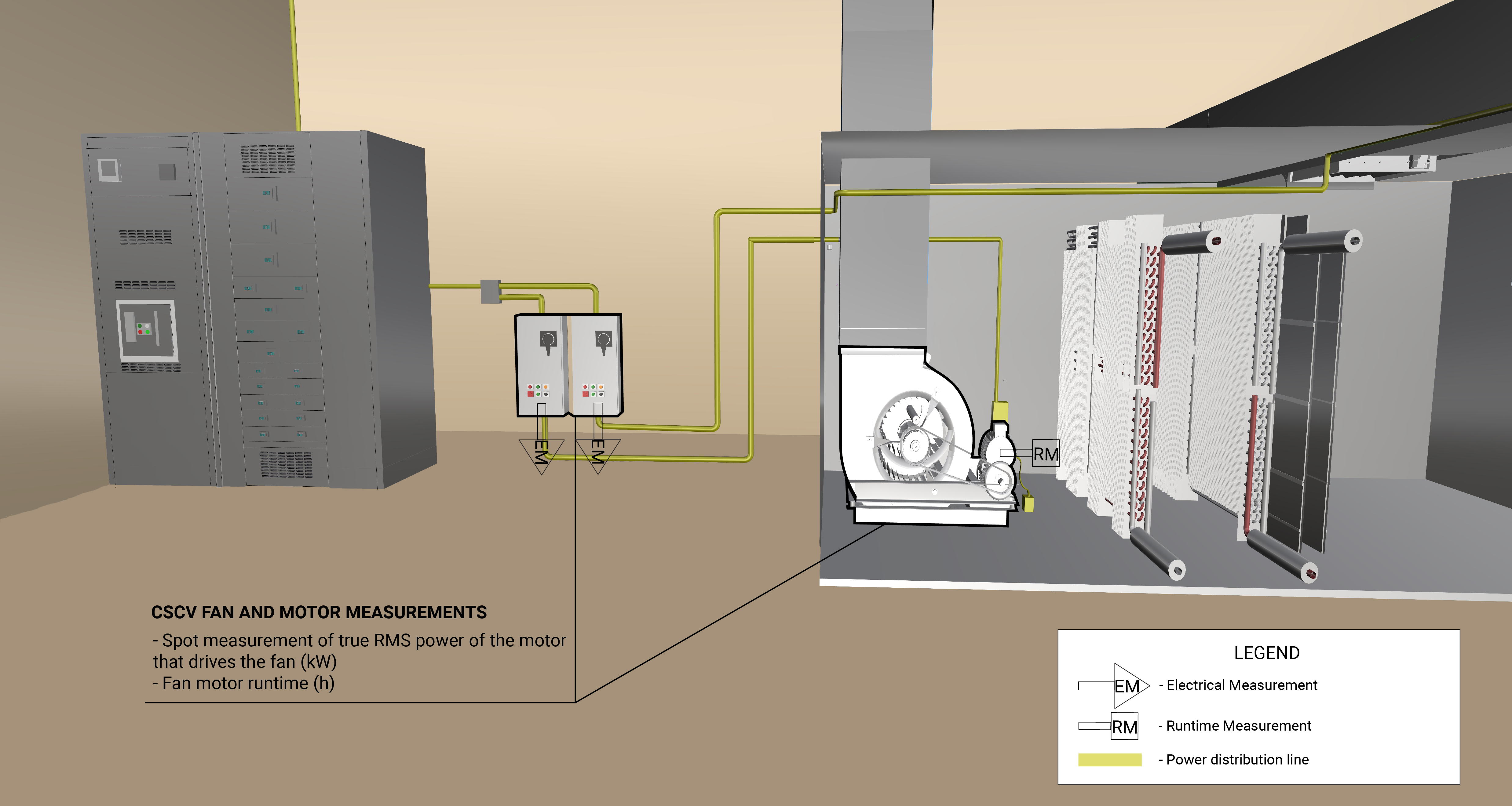
The measurement strategy for a CSCV fan and motor is to take multiple spot measurement of true RMS power and long-term hourly measurements of the operational schedule of the motor. The spot measurements of true RMS power will be averaged and the average value will be used to determine annual energy consumption. True RMS Power is measured at the mainfeed of the panelboard using a handheld power meter. A motor on/off logger is used to measure the hourly motor runtime. Measurement locations are generically represented in Figure 1.
If the fans are in a modular configuration (assuming they all run at the same speed), then only one fan needs to be measured, provided substantiating documentation from the building automation system (BAS) shows that all cells are operating equally at the same time. If fans are further staged, all fans should be measured.
In some cases, the motor’s operational schedule is related to the facility’s heating or cooling load. OAT can serve as a proxy variable for this load and can be measured onsite or obtained from a nearby weather station.
What and How to Measure
Perform the following measurements to quantify the energy consumption and operating characteristics of a CSCV fan and motor:
Measurement Equipment
If you are NYC agency personnel and you’re already familiar with the measurements above, the Field Equipment Lending Library has put together a kit wit all the equipment needed for measuring this component:
Fan and Motor (Constant-Speed) kit
Use this kit to assess the energy consumption (electricity usage) of a constant-speed, constant-volume fan and motor.
Energy Consumption Quantification
The primary energy source for a CSCV fan is the electricity used to run the fan motor. The general methodology for quantifying the energy consumption of a CSCV fan motor involves measuring the true RMS power of the motor. The estimated annual energy consumption of a CSCV fan is estimated using the simulated yearly schedule of the fan. Many CSCV fans run on a set daily or weekly schedule.
However, the yearly schedule may depend on outdoor air temperature (OAT). If so, operating hours can be regressed against OAT to develop a regression model. Depending on operational variability, daily or weekly models may be created to better characterize the component. This model is then applied to climate normal year data to estimate the typical annual operating schedule, which is used alongside true RMS power tUses measured air flow rate, fan power and runtime, and temperature to calculate total annual heat transfer and energy savings for an ERV.o calculate the estimated annual electricity consumption.
How to Quantify
The following downloadable file(s) can be used to calculate energy consumption based on the measurements taken for the specific type of CSCV fan and motor:
For CSCV AHU Supply/Return, Chiller Condenser, and Boiler Burner Fans
Constant Speed Fan Energy Using Motor Runtime Data Calculator
Uses motor runtime (in seconds) and true RMS power (kW) data to estimate annual energy consumption of a CSCV single-speed fan motor.
+More Info
This calculator can work with data from two fans, e.g., if you measured a supply and return fan in an AHU use this calculator to estimate the total annual energy consumption of the AHU. Data from both fans must be in the same format.
Constant One or Two Speed Fan Energy using kW Data Calculator
Uses measured hourly kW data to estimate annual energy consumption for a constant-speed one- or two-speed fan motor.
+More Info
This calculator can work with data from two fans, e.g., if you measured a supply and return fan in an AHU use this calculator to estimate the total annual energy consumption of the AHU. Data from both fans must be in the same format.
For CSCV Cooling Tower (CT) Fans
Further Reading
-
Boyd, BK.; McMordie Stoughton, KL.; Lewis, T. (2017). “Cooling Tower (Evaporative Cooling System) Measurement and Verification Protocol.” Golden, CO: National Renewable Energy Laboratory. https://www.nrel.gov/docs/fy18osti/70219.pdf.
-
Crowther, H.; Furlong, J. (2004). “Optimizing Chillers and Towers.” ASHRAE Journal, Vol. 46, No. 7, July 2004; pp. 34-40.
-
Morrison, F. (2014). “Saving Energy with Cooling Towers.” ASHRAE Journal, Vol. 56, No. 2, February 2014; pp. 34-40.
-
Tom, S. (July 2017). Cat. No. 11-808-616-01. “CHILLED WATER SYSTEM OPTIMIZER.” Farmington, Connecticut: Carrier Corporation.